Like humans, frequency distributions come in different shapes. Immediately after surgery, the majority of patients in the PACU may report ‘no to low’ pain on the Numeric Rating Scale (NRS) that runs from 0 (no pain) to 10 (worst imaginable pain). This NRS frequency distribution, packed with low pain scores and sprinkled with a few moderate or severe pain scores, is positively skewed because it has the appearance of a mound being pulled toward the high end of the distribution. Conversely, several hours after hospital discharge, there may be few patients reporting low pain scores and many patients reporting high pain scores. This NRS frequency distribution is negatively skewed because it has the appearance of a mound being pulled toward the low end of the distribution. Many things in nature are distributed in a bell shape – blood pressure, pulse rate, salt consumption, and so forth – but there is only one standard normal or Gaussian curve, named for Carl Friedrich Gauss, a German mathematician (1777-1855).

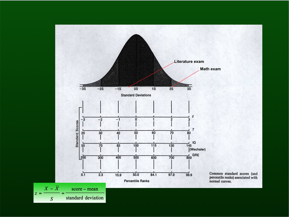
Besides having a symmetrical bell shape, this curve has mean 0 and standard deviation (s.d.) 1. The left and right tails of this curve do not touch the horizontal line because they go to negative and positive infinity, respectively. Approximately 68% of scores fall within ±1 s.d. of the mean, 95% of scores fall within ±1.96 s.d. of the mean, and virtually all scores fall within ±3 s.d. of the mean. These characteristics allow us to determine “addresses” or standard z scores that can be compared across measures. So, for instance, the child who happily reports a score of 98 on a literature exam (say, z = -0.5), but sadly reports a score of 69 on a math exam (say, z = 2.1), actually did rather mediocre on the literature exam but was quite exceptional on the math exam!

But what does this have to do with statistical testing of a mean or mean difference? A simple calculation of a standard (z) score gives us its position on the normal curve, and we can use this address to evaluate the rarity of the mean or mean difference that we are investigating in a research study. Does our mean or mean difference have a mediocre or an exceptional address? Simply put, findings with mediocre z scores in the middle of the distribution occur frequently while those with exceptional z scores in the tails of the distribution occur infrequently. This frame of reference was brought to you through the courtesy of the one and only Gaussian curve! It is fitting that next month we end the first year of Statistics in Small Doses with a discussion of p-values.