


The basic principles of pharmacology are a fundamental element of an anesthesia provider’s knowledge base. This chapter provides an overview of key principles in clinical pharmacology used to describe anesthetic drug behavior. Box 1 lists definitions of some basic pharmacologic terms. Pharmacokinetic concepts include volumes of distribution, drug clearance, transfer of drugs between plasma and tissues, and binding of drugs to circulating plasma proteins. The section on pharmacokinetics introduces both the physiologic processes that determine pharmacokinetics and the mathematical models used to relate dose to concentration. Anesthesia providers rarely administer just one drug. Most anesthetics are a combination of several drugs with specific goals in analgesia, sedation, and muscle relaxation. Thus, pharmacodynamic interactions can profoundly influence anesthetic effect. Formulating the right dose of an anesthetic requires consideration of many patient factors: age; body habitus; sex; chronic exposure to opioids, benzodiazepines, or alcohol; presence of heart, lung, kidney, or liver disease; and the extent of blood loss or dehydration, among others. Two of these factors, body habitus and age, will be discussed as examples of patient factors influencing anesthetic drug pharmacology.
1. PHARMACOKINETIC PRINCIPLES
Pharmacokinetics describes the relationship between drug dose and drug concentration in plasma or at the site of drug effect over time. The processes of absorption, distribution, and elimination (metabolism and excretion) govern this relationship. Absorption is not relevant to intravenously administered drugs but is relevant to all other routes of drug delivery. The time course of intravenously administered drugs is a function of distribution volume and clearance. Estimates of distribution volumes and clearances are described by pharmacokinetic parameters. Pharmacokinetic parameters are derived from mathematical formulas fit to measured blood or plasma concentrations over time following a known drug dose.
Fundamental Pharmacokinetic Concepts
Volume of Distribution
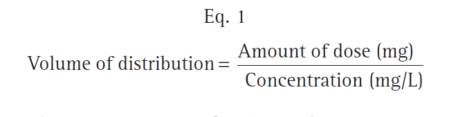
An oversimplified model of drug distribution throughout plasma and tissues is the dilution of a drug dose into a tank of water. The volume of distribution (Vd) is the apparent size of the tank required to explain a measured drug concentration from the tank water once the drug has had enough time to thoroughly mix within the tank (Fig. 1). The distribution volume is estimated using the simple relationship between dose (e.g., mg) and measured concentration (e.g., mg/L) as presented in Eq. 1.

- Fig. 1 Schematic of a single-tank model of distribution volume. The group of red dots at the top left represent a bolus dose that, when administered to the tank of water, evenly distribute within the tank. (Modified from Miller RD, Cohen NH, Eriksson LI, et al, eds. Miller’s Anesthesia. 8th ed. Philadelphia: Saunders Elsevier; 2014: Fig. 1.)
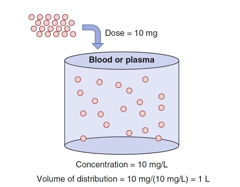
With an estimate of tank volume, drug concentration after any bolus dose can be calculated. Just as the tank has a volume regardless of whether there is drug in it, distribution volumes in people are an intrinsic property regardless of whether any drug has been given.
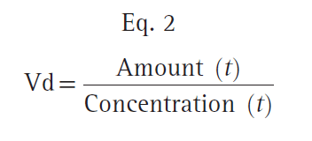
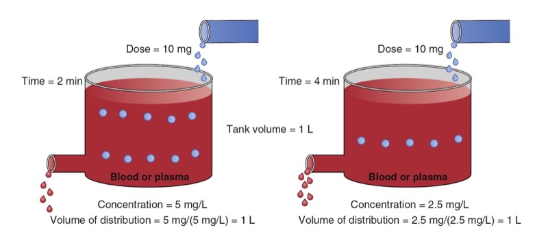
Human bodies are not water tanks. As soon as a drug is injected, it begins to be cleared from the body. To account for this in the schematic presented in Fig. 1, a faucet is added to the tank to mimic drug elimination from the body (Fig. 2). Using Eq. 1, estimating the volume of distribution without accounting for elimination leads to volume of distribution estimates that become larger than initial volume. To refine the definition of distribution volume, the amount of drug that is present at a given time t is divided by the concentrations at the same time.

- Fig. 2 Schematic of a single-tank model of elimination as a first-order process. At 2 minutes (left panel) and 4 minutes (right panel) following a 10-mg drug bolus, tank concentrations are decreasing from 5 to 2.5 mg/mL. Accounting for elimination, estimates of the distribution volume at each time point are both 1 L. (From Miller RD, Cohen NH, Eriksson LI, et al, eds. Miller’s Anesthesia. 8th ed. Philadelphia: Saunders Elsevier; 2014: Fig. 2.)

- Fig. 3 Simulation of concentration (left) and distribution volume (right) changes over time following a bolus dose for a single-tank (one-compartment) model. The distribution volume remains constant throughout. (From Miller RD, Cohen NH, Eriksson LI, et al, eds. Miller’s Anesthesia. 8th ed. Philadelphia: Saunders Elsevier; 2014: Fig. 3.)
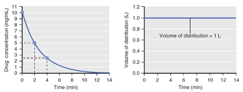
If elimination occurs as a first-order process (i.e., elimination is proportional to the concentration at that time), the volume of distribution calculated by Eq. 2 will be constant (Figs. 2 and 3).
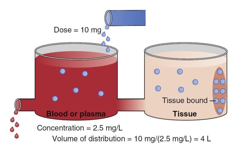
When a drug is administered intravenously, some drug stays in the vascular volume, but most of the drug distributes to peripheral tissues. This distribution is often represented as additional volumes of distribution (tanks) connected to a central tank (blood or plasma volume). Peripheral distribution volumes increase the total volume of distribution (Fig. 4).
The schematic in Fig. 4 presents a plasma volume and tissue volume. The peripheral tank represents distribution of drug in peripheral tissues. There may be more than one peripheral tank (volume) to best describe the entire drug disposition in the body. The size of the peripheral volumes represents a drug’s solubility in tissue relative to blood or plasma. The more soluble a drug is in peripheral tissue relative to blood or plasma, the larger the peripheral volumes of distribution.
An important point illustrated in Fig. 4 is that drug not only distributes to the peripheral tank and thus increases the volume of distribution, but it also binds to tissue in that tank. This process further lowers the measurable concentration in the central tank. Thus, the total volume of distribution may even be larger than the two tanks added together. In fact, some anesthetics have huge distribution volumes (e.g., fentanyl has an apparent distribution volume of 4 L/ kg) that are substantially larger than an individual’s vascular volume (0.07 L/kg) or extracellular volume (0.2 L/kg).

- Fig. 4 Schematic of a two-tank model. The total volume of distribution consists of the sum of the two tanks. The blue dots in the ellipse in the peripheral volume represent tissue-bound drug. The measured concentration in the blood or plasma is 2.5 mg/ mL just after a bolus dose of 10 mg. Using Fig. 1, this leads to a distribution volume of 4 L. (From Miller RD, Cohen NH, Eriksson LI, et al, eds. Miller’s Anesthesia. 8th ed. Philadelphia: Saunders Elsevier; 2015: Fig. 4.)
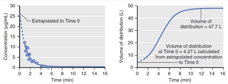
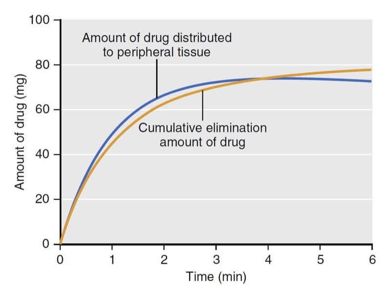
With an additional tank, the volume of distribution no longer remains constant over time. As illustrated in Fig. 5, at time = 0, the volume of distribution is estimated as 4.3 L, the same as that of the model presented in Fig. 3, which has only one tank. The volume of distribution then increases to 48 L over the next 10 minutes. The increase is due to the distribution of drug to the peripheral volume and elimination once drug is in the body. The amount of drug that moves to the peripheral tissue commonly surpasses the amount that is eliminated during the first few minutes after drug administration. As an example, consider a simulation of a propofol bolus that plots the accumulation of propofol in peripheral tissues and the amount eliminated over time (Fig. 6). During the first 4 minutes, the amount distributed to the peripheral tissue is larger than the amount eliminated from the body. Following 4 minutes, the amounts reverse.

- Fig.5 Simulation of concentration and apparent distribution volume changes over time following a bolus dose for a two-tank (two-compartment) model. On the left, the dots represent measured drug concentrations. The solid line represents a mathematical equation fit to the measured concentrations. The dotted line represents an extrapolation of the mathematical equation (i.e., pharmacokinetic model) to time 0. On the right, the apparent distribution volume is time dependent with the initial volume of distribution much smaller than the distribution volume at near steady state. The apparent distribution volume of time 0 is not a true reflection of the actual volume of distribution. (From Miller RD, Cohen NH, Eriksson LI, et al, eds. Miller’s Anesthesia. 8th ed. Philadelphia: Saunders Elsevier; 2015: Fig. 5.)

- Fig. 6 Simulation of propofol accumulation in the peripheral tissues (blue line) and the cumulative amount of propofol eliminated (yellow line) following a 2-mg/kg propofol bolus to a 77-kg (170-lb), 177-cm (5 ft 10 in) tall, 53-year-old man, using published pharmacokinetic model parameters.1 Drug indicates propofol. (From Miller RD, Cohen NH, Eriksson LI, et al, eds. Miller’s Anesthesia. 8th ed. Philadelphia: Saunders Elsevier; 2015: Fig. 6.)
Clearance
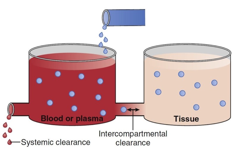
Clearance describes the rate of drug removal from the plasma/blood. Two processes contribute to drug clearance: systemic (out of the tank) and intercompartmental (between the tanks) clearance (Fig. 7). Systemic clearance permanently removes drug from the body, either by eliminating the parent molecule or by transforming it into metabolites. Intercompartmental clearance moves drug between plasma and peripheral tissue tanks. By way of clarification, in this chapter the words compartment and tank are used interchangeably.

- Fig. 7 Schematic of a two-tank model illustrating two sources of drug removal from the central tank (blood or plasma): systemic and intercompartmental clearance. (From Miller RD, Cohen NH, Eriksson LI, et al, eds. Miller’s Anesthesia. 8th ed. Philadelphia: Saunders Elsevier; 2015: Fig. 8.)
Clearance is defined in units of flow, that is, the volume completely cleared of drug per unit of time (e.g., L/ min). Clearance is not to be confused with elimination rate (e.g., mg/min). To explain why elimination rates do lation
presented in Fig. 8.

- Fig. 8 Simulation of drug concentration changes when a drug is administered to a single-tank model with linear elimination (see Fig. 2). The concentration changes for two time windows are labeled with diagonal lines from 1 to 2 minutes (time window A) and from 3 to 4 minutes (time window B), respectively. The concentrations (CON) at the beginning and end of each time window are used to calculate the amount (AMT) of drug that is eliminated (see text). Vd, Volume of distribution. (Modified from Miller RD, Cohen NH, Eriksson LI, et al, eds. Miller’s Anesthesia. 8th ed. Philadelphia: Saunders Elsevier; 2015: Fig. 9.)
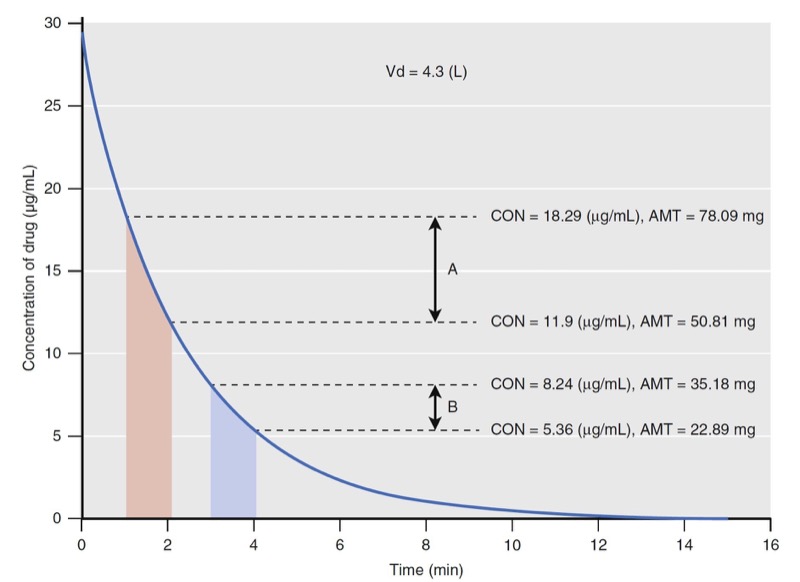
Using the volume of distribution, the total amount of drug can be calculated at every measured drug concentration. The concentration change in time window A is larger than that in time window B even though they are both 1 minute in duration. The elimination rates are 27 and 12 mg/min for time windows A and B, respectively. They are different and neither can be used as a parameter to predict drug concentrations when another dose of drug is administered. Because of this limitation with elimination rate, clearance was developed to provide a single number to describe the decay in drug concentration presented in Fig. 8.
For discussion purposes, assume that concentration is the power necessary to push drug out of the water tank. The higher the concentration, the larger the amount of drug eliminated. To standardize the elimination rate, the eliminated amount of drug is scaled to concentration. For example, the elimination rate in time window A (27 mg/ min) scaled to the mean concentration during that time window (15 μg/mL) is 0.001807 mg/min/mg/L. Reducing the units gives 0.002 L/min. Normalizing the elimination rate in time window B to concentration gives the same result as A. If the time interval is narrowed so that the time window approaches zero, the definition of clearance becomes:
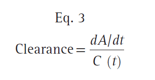
where dA/dt is the rate of drug elimination at given time t, and C (t) is the corresponding concentration at time t. Rearranging Eq. 3, clearance can be expressed as follows:
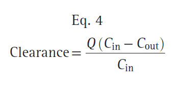
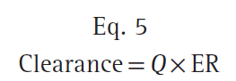
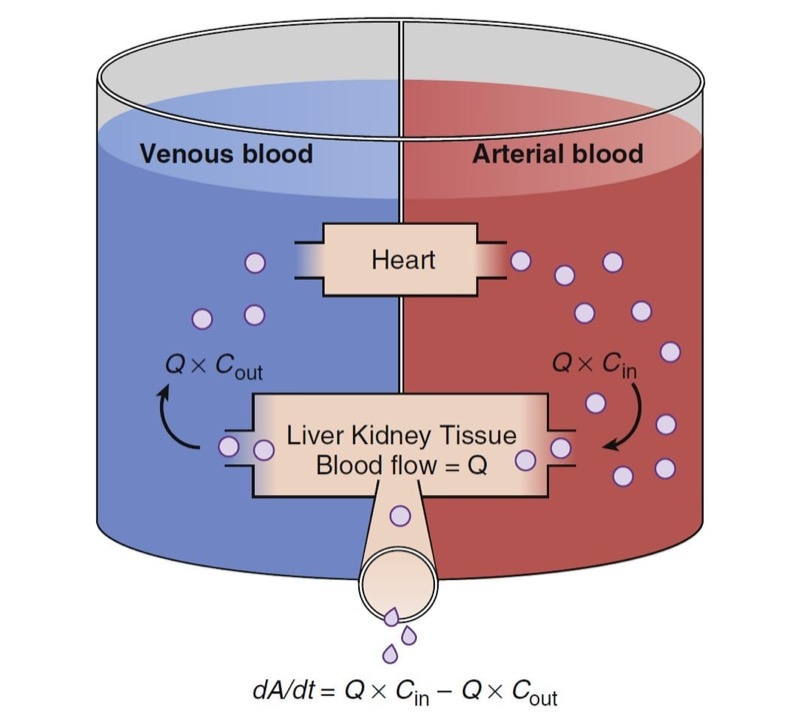
where Q is the blood flow to metabolic organs, Cin is the concentration of drug delivered to metabolic organs, and Cout is the concentration of drug leaving metabolic organs. The fraction of inflowing drug extracted by the organ is (Cin − Cout)/Cin and is called the extraction ratio (ER). Clearance can be estimated as organ blood flow multiplied by the ER. Eq. 4 can be simplified as shown here:
The total clearance is the sum of each clearance by metabolic organs such as the liver, kidney, and other tissues (Fig. 9).

- Fig. 9 Schematic of drug extraction. A, Amount of drug; Cin and Cout, drug concentrations presented to and leaving metabolic organs; dA/dt, drug elimination rate; Q, blood flow. (From Miller RD, Cohen NH, Eriksson LI, et al, eds. Miller’s Anesthesia. 8th ed. Philadelphia: Saunders Elsevier; 2015: Fig. 10.)
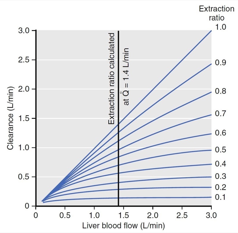
Hepatic clearance has been well characterized. For example, the relationship between clearance, liver blood flow, and the extraction ratio is presented in Fig. 10. (2) For drugs with an extraction ratio of nearly 1 (e.g., propofol), a change in liver blood flow produces a nearly proportional change in clearance. For drugs with a low extraction ratio (e.g., alfentanil), clearance is nearly independent of the rate of liver blood flow. If nearly 100% of the drug is extracted by the liver, this implies that the liver has tremendous metabolic capacity for the drug. In this case, the rate-limiting step in metabolism is flow of drug to the liver, and such drugs are said to be “flow limited.” Any reduction in liver blood flow, such as usually accompanies anesthesia, can be expected to reduce clearance. However, moderate changes in hepatic metabolic function per se will have little impact on clearance because hepatic metabolic capacity is overwhelmingly in excess of demand.
For many drugs (e.g., alfentanil), the extraction ratio is considerably less than 1. For these drugs, clearance is limited by the capacity of the liver to take up and metabolize drug. These drugs are said to be “capacity limited.” Clearance will change in response to any change in the capacity of the liver to metabolize such drugs, as might be caused by liver disease or enzymatic induction. However, changes in liver blood flow, as might be caused by the anesthetic state itself, usually have little influence on clearance because the liver handles only a fraction of the drug that it sees anyway.

- Fig.10 Relationship among liver blood flow (Q), clearance, and extraction ratio. For drugs with a high extraction ratio, clearance is nearly identical to liver blood flow. For drugs with a low extraction ratio, changes in liver blood flow have almost no effect on clearance.2 (From Miller RD, Cohen NH, Eriksson LI, et al, eds. Miller’s Anesthesia. 8th ed. Philadelphia: Saunders Elsevier; 2015: Fig.11.)
Front-End Kinetics
Front-end kinetics refers to the description of intravenous drug behavior immediately following administration. How rapidly a drug moves from the blood into peripheral tissues directly influences the peak plasma drug concentration. With compartmental models, an important assumption is that an intravenous bolus instantly mixes in the central volume, with the peak concentration occurring at the moment of injection without elimination or distribution to peripheral tissues. For simulation purposes, the initial concentration and volume of distribution at time = 0 are extrapolated as if the circulation had been infinitely fast. This, of course, is not real. If drug is injected into an arm vein and that initial concentration is measured in a radial artery, drug appears in the arterial circulation 30 to 40 seconds after injection. The delay likely represents the time required for drug to pass through the venous volume of the upper part of the arm, heart, great vessels, and peripheral arterial circulation. More sophisticated models (e.g., a recirculatory model)3 account for this delay and are useful when characterizing the behavior of a drug immediately following bolus administration, such as with induction agents, when the speed of onset and duration of action are of interest.
Compartmental Pharmacokinetic Models
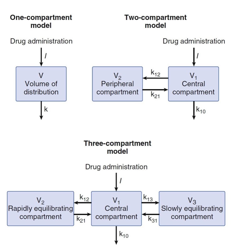
Compartmental models have no physiologic correlate. They are built by using mathematical expressions fit to concentration over time data and then reparameterized in terms of volumes and clearances. The one-compartment model presented in Fig. 11 contains a single volume and a single clearance. Although used for several drugs, this model is perhaps oversimplified for anesthetic drugs. To better model anesthetic drugs, clinical pharmacologists have developed two or three compartment models that contain several tanks connected by pipes. As illustrated in Fig. 11, the volume to the right in the two-compartment model—and in the center of the three-compartment model—is the central volume. The other volumes are peripheral volumes. The sum of the all volumes is the volume of distribution at steady state, Vdss. Clearance in which the central compartment is left for the outside is the central or metabolic clearance. Clearances between the central compartment and the peripheral compartments are the intercompartmental clearances.

- Fig. 11 One-, two-, and three-compartment mammillary models. (From Miller RD, Cohen NH, Eriksson LI, et al, eds. Miller’s Anesthesia. 8th ed. Philadelphia: Saunders Elsevier; 2015: Fig. 12.)
Multicompartment Models
Plasma concentrations over time after an intravenous bolus resemble the curve in Fig. 12. This curve has the characteristics common to most drugs when given as an intravenous bolus. First, the concentrations continuously decrease over time. Second, the rate of decline is initially steep but continuously becomes less steep, until we get to a portion that is log-linear.
For many drugs, three distinct phases can be distinguished, as illustrated for fentanyl in Fig. 12. A rapid-distribution phase (blue line) begins immediately after injection of the bolus. Very rapid movement of the drug from plasma to the rapidly equilibrating tissues characterizes this phase. Next, a second slowdistribution phase (red line) is characterized by movement of drug into more slowly equilibrating tissues and return of drug to plasma from the most rapidly equilibrating tissues. Third, the terminal phase (green line) is nearly a straight line when plotted on a semilogarithmic graph. The terminal phase is often called the “elimination phase” because the primary mechanism for decreasing drug concentration during the terminal phase is elimination of drug from the body. The distinguishing characteristic of the terminal elimination phase is that the plasma concentration is lower than tissue concentrations and the relative proportion of drug in plasma and peripheral volumes of distribution remains constant. During this terminal phase, drug returns from the rapid- and slow-distribution volumes to plasma and is permanently removed from plasma by metabolism or excretion.

- Fig.12 Hydraulic model of fentanyl pharmacokinetics. Drug is administered into the central tank, from which it can distribute into two peripheral tanks, or it may be eliminated. The volume of the tanks is proportional to the volumes of distribution. The cross-sectional area of the pipes is proportional to clearance.4 (From Miller RD, Cohen NH, Eriksson LI, et al, eds. Miller’s Anesthesia. 8th ed. Philadelphia: Saunders Elsevier; 2015: Fig.13.)
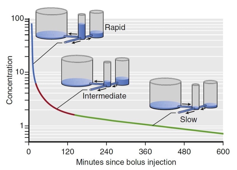
The presence of three distinct phases after bolus injection is a defining characteristic of a mammillary model with three compartments.4 In this model, shown in Fig. 12, there are three tanks corresponding (from left to right) to the slowly equilibrating peripheral compartment, the central compartment (the plasma, into which drug is injected), and the rapidly equilibrating peripheral compartment. The horizontal pipes represent intercompartmental clearance or (for the pipe draining onto the page) metabolic clearance. The volumes of each tank correspond to the volumes of the compartments for fentanyl. The cross-sectional areas of the pipes correlate with fentanyl systemic and intercompartmental clearance. The height of water in each tank corresponds to drug concentration. By using this hydraulic model we can follow the processes that decrease drug concentration over time after bolus injection. Initially, drug flows from the central compartment to both peripheral compartments via intercompartmental clearance and completely out of the model via metabolic clearance. Because there are three places for drug to go, the concentration in the central compartment decreases very rapidly. At the transition between the blue line and the red line, there is a change in the role of the most rapidly equilibrating compartment. At this transition, the concentration in the central compartment falls below the concentration in the rapidly equilibrating compartment, and the direction of flow between them is reversed. After this transition (red line), drug in plasma has only two places to go: into the slowly equilibrating compartment or out the drain pipe. These processes are partly offset by the return of drug to plasma from the rapidly equilibrating compartment. The net effect is that once the rapidly equilibrating compartment has come to equilibration, the concentration in the central compartment falls far more slowly than before.
Once the concentration in the central compartment decreases below both the rapidly and slowly equilibrating compartments (green line), the only method of decreasing the plasma concentration is metabolic clearance, the drain pipe. Return of drug from both peripheral compartments to the central compartment greatly slows the rate of decrease in plasma drug concentration. Curves that continuously decrease over time, with a continuously increasing slope (i.e., like the curve in Fig. 12), can be described by a sum of negative exponentials. In pharmacokinetics, one way of denoting this sum of exponentials is to say that the plasma concentration over time is as follows:

where t is the time since the bolus injection, C (t) is the drug concentration after a bolus dose, and A, α, B, β, C, and γ are parameters of a pharmacokinetic model. A, B, and C are coefficients, whereas α, β, and γ are exponents. After a bolus injection, all six of the parameters in Eq. 6 will be greater than 0. Polyexponential equations are used mainly because they describe the plasma concentrations observed after bolus injection, except for the misspecification in the first few minutes, mentioned previously. Compartmental pharmacokinetic models are strictly empiric. These models have no anatomic correlate. They are based solely on fitting equations to measured plasma concentrations following a known dose. Kinetic models are transformed into models that characterize concentration changes over time in terms of volumes and clearances. Although more intuitive, they have no physiologic correlate.
Special significance is often ascribed to the smallest exponent. This exponent determines the slope of the final log-linear portion of the curve. When the medical literature refers to the half-life of a drug, unless otherwise stated, the half-life will be the terminal half-life. However, the terminal half-life for drugs with more than one exponential term is nearly uninterpretable. The terminal half-life sets an upper limit on the time required for the concentrations to decrease by 50% after drug administration. Usually, the time needed for a 50% decrease will be much faster than that upper limit.
Part of the continuing popularity of pharmacokinetic compartmental models is that they can be transformed from an unintuitive exponential form to a more intuitive compartmental form, as shown in Fig.11. Microrate constants, expressed as kij, define the rate of drug transfer from compartment i to compartment j. Compartment 0 is the compartment outside the model, so k10 is the microrate constant for processes acting through metabolism or elimination that irreversibly remove drug from the central compartment (analogous to k for a onecompartment model). The intercompartmental microrate constants (k12, k21, etc.) describe movement of drug between the central and peripheral compartments. Each peripheral compartment has at least two microrate constants, one for drug entry and one for drug exit. The microrate constants for the two- and three-compartment models can be seen in Fig. 11.
Back-End Kinetics
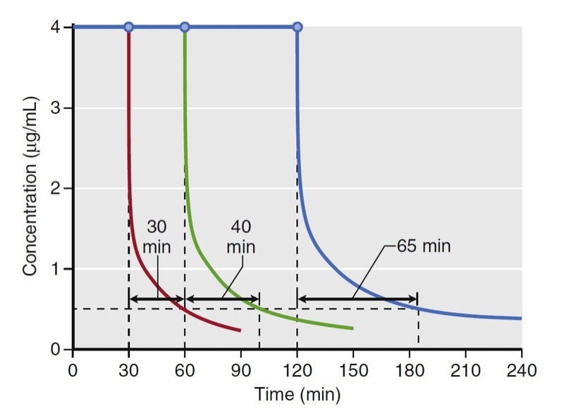
Using estimates of distribution volume and clearance, back-end kinetics is a useful tool that describes the behavior of intravenous drugs when administered as continuous infusions. Back-end kinetics provides descriptors of how plasma drug concentrations decrease once a continuous infusion is terminated. An example is decrement time. It predicts the time required to reach a certain plasma concentration once an infusion is terminated. Decrement times are a function of infusion duration. Consider the example of decrement times for a set of continuous target-controlled infusions (Fig. 13). In this simulation, target-controlled infusion (TCI) of propofol is set to maintain a concentration of 4 μg/mL for 30, 60, and 120 minutes. Once the infusion is stopped, the time to reach 0.5 μg/mL is estimated. As illustrated, the longer the infusion, the longer the time required to reach 0.5 μg/ mL. This example demonstrates how drugs accumulate in peripheral tissues with prolonged infusions. This accumulation prolongs the decrement time.

- Fig. 13 Simulation of decrement times for a target-controlled infusion set to maintain a target propofol concentration of 4 μg/ mL for 30, 60, and 120 minutes. Once terminated, the time required to reach 0.5 μg/mL was 30, 40, and 65 minutes for each infusion, respectively. Simulations of the decrement times used a published pharmacokinetic model.1 (From Miller RD, Cohen NH, Eriksson LI, et al, eds. Miller’s Anesthesia. 8th ed. Philadelphia: Saunders Elsevier; 2015: Fig. 14.)
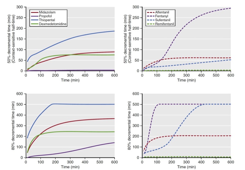
Another use of decrement times is as a tool to compare drugs within a drug class (e.g., opioids). As a comparator, plots of decrement times are presented as a function of infusion duration. When used this way, decrement times are determined as the time required to reach a target percentage of the concentration immediately after termination of a continuous infusion. Examples of 50% and 80% decrement times for selected opioids and sedatives are presented in Fig. 14. Of note, for shorter infusions, the decrement times are similar for both classes of anesthetic drugs. Once infusion duration exceeds 2 hours, the decrement times vary substantially. A popular decrement time is the 50% decrement time, also known as the context-sensitive halftime. (5) The term context-sensitive refers to infusion duration. The term half-time refers to the 50% decrement time.

- Fig. 14 These graphs show 50% and 80% decrement times for selected sedatives (left side) and opioids (right side). The vertical axis refers to the time required to reach the desired decrement time. The horizontal axis refers to infusion duration. Simulations of the decrement times used published pharmacokinetic models for each sedative and analgesic.5-10 (From Miller RD, Cohen NH, Eriksson LI, et al, eds. Miller’s Anesthesia. 8th ed. Philadelphia: Saunders Elsevier; 2015: Fig.15.)
Biophase
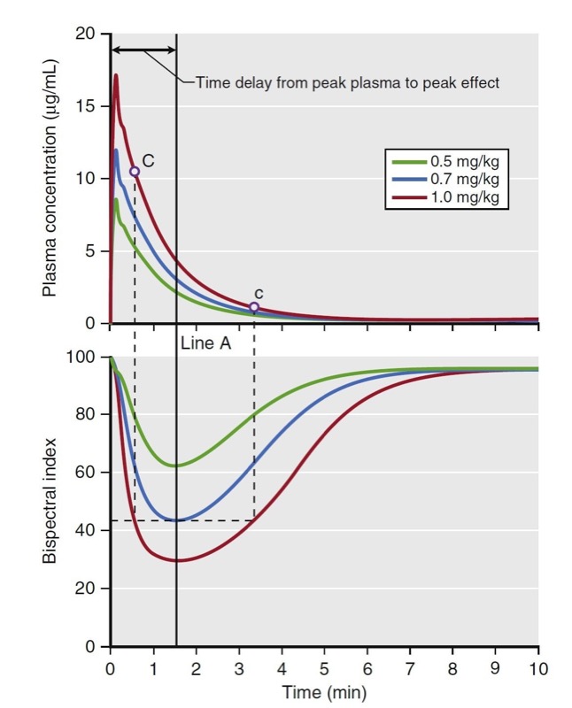
Biophase refers to the time delay between changes in plasma concentration and drug effect. Biophase accounts for the time required for drug to diffuse from the plasma to the site of action plus the time required, once drug is at the site of action, to elicit a drug effect. A simulation of various propofol bolus doses and their predicted effect on the electroencephalogram (EEG) bispectral index scale (BIS) is presented in Fig. 15. The time to peak effect for each dose is identical (approximately 1.5 minutes following the peak plasma concentration). The difference between each dose is the magnitude and duration of effect. A key principle is that when drug concentrations are in flux (i.e., during induction of anesthesia and emergence from anesthesia), changes in drug effect will lag behind changes in drug concentration. This lag between the plasma concentration and effect usually results in the phenomenon called hysteresis, in which two different plasma concentrations correspond to one drug effect or one plasma concentration corresponds to two drug effects. For example, Fig. 15 shows that the different concentrations at C and c correspond to the same BIS score.

- Fig.15 Demonstration of biophase. The top plot presents a simulation of three propofol doses and the resultant plasma concentrations. The bottom plot presents a simulation of the predicted effect on the bispectral index scale (BIS). These simulations assume linear kinetics: regardless of the dose, effects peak at the same time (Line A), as do the plasma concentration. The time to peak effect is 1.5 minutes. Even the plasma concentrations of points C and c are different; however, the BIS scores of those two points are the same. This finding demonstrates the hysteresis between plasma concentration and BIS score. Simulations used published pharmacokinetic and pharmacodynamic models.1,7 (From Miller RD, Cohen NH, Eriksson LI, et al, eds. Miller’s Anesthesia. 8th ed. Philadelphia: Saunders Elsevier; 2015: Fig.16.)
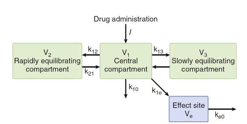
To collapse the hysteresis between plasma concentration and effect and to match one plasma concentration to one drug effect, this lag is often modeled with an “effect site” compartment added to the central compartment. Kinetic microrate constants used to describe biophase include k1e and ke0. The k1e describes drug movement from the central compartment to the effect site and ke0 describes the elimination of drug from the effect site compartment. There are two important assumptions with the effect-site compartment: (1) The amount of drug that moves from the central compartment to the effect-site compartment is negligible and vice versa, and (2) there is no volume estimate to the effect-site compartment.
Typically, the relationship between plasma and the site of drug effect is modeled with an effect-site model, as shown in Fig. 16. The site of drug effect is connected to plasma by a first-order process. Eq. 7 relates effect-site concentration to plasma concentration:
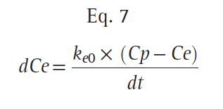
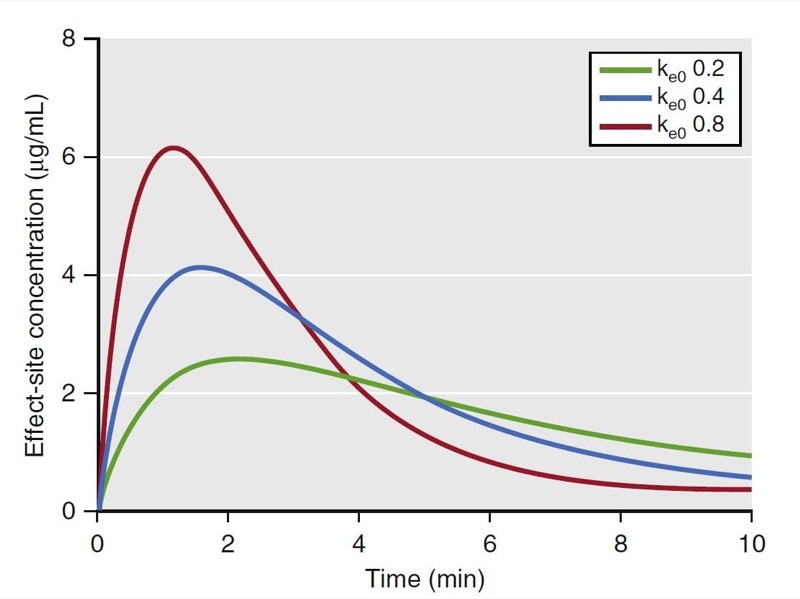
where Ce is the effect-site concentration, Cp is the plasma drug concentration, and ke0 is the rate constant for elimination of drug. The constant ke0 describes the rate of rise and offset of drug effect (Fig. 17).
In summary, the conventional pharmacokinetic term half-life has little meaning to anesthesia providers, who work with drugs whose clinical behavior is not well described by half-life. The pharmacokinetic principles discussed in this section (such as volume of distribution, clearance, elimination, front-end kinetics, back-end kinetics, context-sensitive half-time, and biophase) better illustrate how an anesthetic will behave.

- Fig. 16 A three-compartment model with an added effect site to account for the delay in equilibration between the rise and fall in arterial drug concentrations and the onset and offset of drug effect. The effect site is assumed to have a negligible volume. (From Miller RD, Cohen NH, Eriksson LI, et al, eds. Miller’s Anesthesia. 8th ed. Philadelphia: Saunders Elsevier; 2015 :Fig. 17.)

- Fig.17 Effect of the ke0 changes. As the ke0 decreases, the time to peak effect is prolonged. (1,7,11) (From Miller RD, Cohen NH, Eriksson LI, et al, eds. Miller’s Anesthesia. 8th ed. Philadelphia: Saunders Elsevier; 2015: Fig. 18.)
2. PHARMACODYNAMIC PRINCIPLES
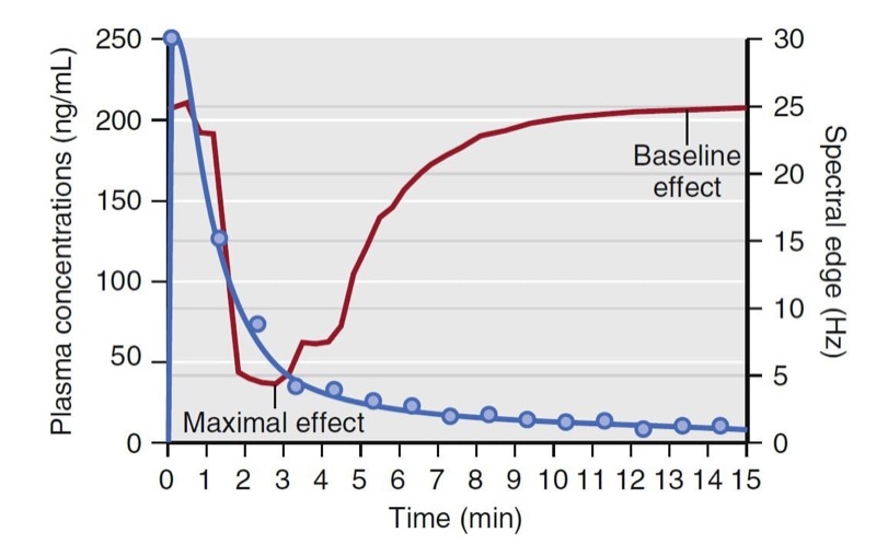
Simply stated, pharmacokinetics describes what the body does to the drug, whereas pharmacodynamics describes what the drug does to the body. In particular, pharmacodynamics describes the relationship between drug concentration and pharmacologic effect. Models used to describe the concentration-effect relationships are created in much the same way as pharmacokinetic models; they are based on observations and used to create a mathematical model. To create a pharmacodynamic model, plasma drug levels and a selected drug effect are measured simultaneously. For example, consider the measured plasma concentrations of an intravenous anesthetic drug following a bolus dose and the associated changes on the EEG spectral edge frequency (a measure of anesthetic depth) from one individual, presented in Fig. 18. Shortly after the plasma concentration peaks, the spectral edge starts to decrease, reaches a nadir, and then returns back to baseline as the plasma concentrations drop to near 0.

- Fig. 18 Schematic representation of drug plasma concentrations (blue circles) following a bolus and the associated changes in the electroencephalogram’s spectral edge (red line) measured in one individual. Note that changes in spectral edge lag behind changes in plasma concentrations. (From Miller RD, Cohen NH, Eriksson LI, et al, eds. Miller’s Anesthesia. 8th ed. Philadelphia: Saunders Elsevier; 2015: Fig.19.)
Combining data from several individuals and plotting the measured concentrations versus the observed effect (modified to be a percentage of the maximal effect across all individuals) creates a hysteresis loop (Fig.19). The ascending portion of the loop represents rising drug concentrations (see arrow). While rising, the increase in drug effect lags behind the increase in drug concentration. For the descending loop, the decrease drug effect lags behind the decrease in drug concentration.

- Fig. 19 Schematic representation of plasma concentrations versus normalized spectral edge measurements (presented as a percentage of maximal effect) from several individuals (blue circles). The black arrows indicate the ascending and descending arms of a hysteresis loop that coincide with increasing and decreasing drug concentrations. The red line represents the pharmacodynamic model developed from collapsing the hysteresis loop. EEG, electroencephalogram. (From Miller RD, Cohen NH, Eriksson LI, et al, eds. Miller’s Anesthesia. 8th ed. Philadelphia: Saunders Elsevier; 2015: Fig. 20.)
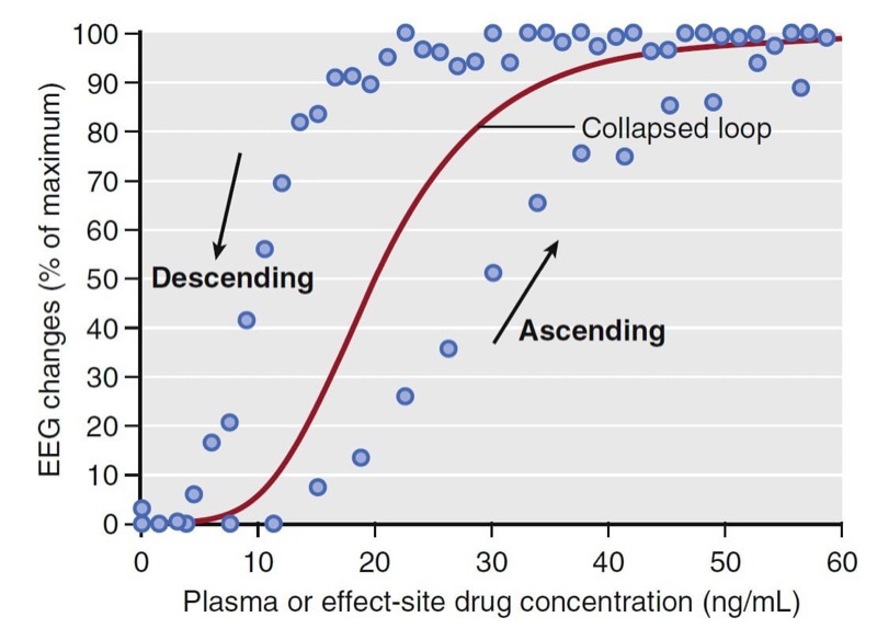
To create a pharmacodynamic model, the hysteresis loop is collapsed using modeling techniques that account for the lag time between plasma concentrations and the observed effect. These modeling techniques provide an estimate of the lag time, known as the t½ke0, and an estimate of the effect-site concentration (Ce) associated with a 50% probability of drug effect (C50). Most concentration- effect relationships in anesthesia are described with a sigmoid curve. The standard equation for this relationship is the Hill equation, also known as the sigmoid Emax relationship (Eq. 8):
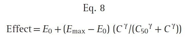
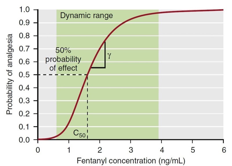
where E0 is the baseline effect, Emax is the maximal effect, C is the drug concentration, and γ represents the slope of the concentration-effect relationship; γ is also known as the Hill coefficient. For values of γ less than 1, the curve is hyperbolic, and for values greater than 1, the curve is sigmoid. Fig. 20 presents an example of this relationship: a fentanyl effect-site concentration-effect curve for analgesia. This example illustrates how C50 and γ characterize the concentration-effect relationship.

- Fig. 20 A pharmacodynamic model for the analgesic effect of fentanyl. The green area represents the dynamic range, the concentration range where changes in concentration lead to a change in effect. Concentrations above or below the dynamic range do not lead to changes in drug effect. The C50 represents the concentration associated with 50% probability of analgesia. Gamma (γ) represents the slope of the curve in the dynamic range. (From Miller RD, Cohen NH, Eriksson LI, et al, eds. Miller’s Anesthesia. 8th ed. Philadelphia: Saunders Elsevier; 2015: Fig. 21.)
Potency and Efficacy
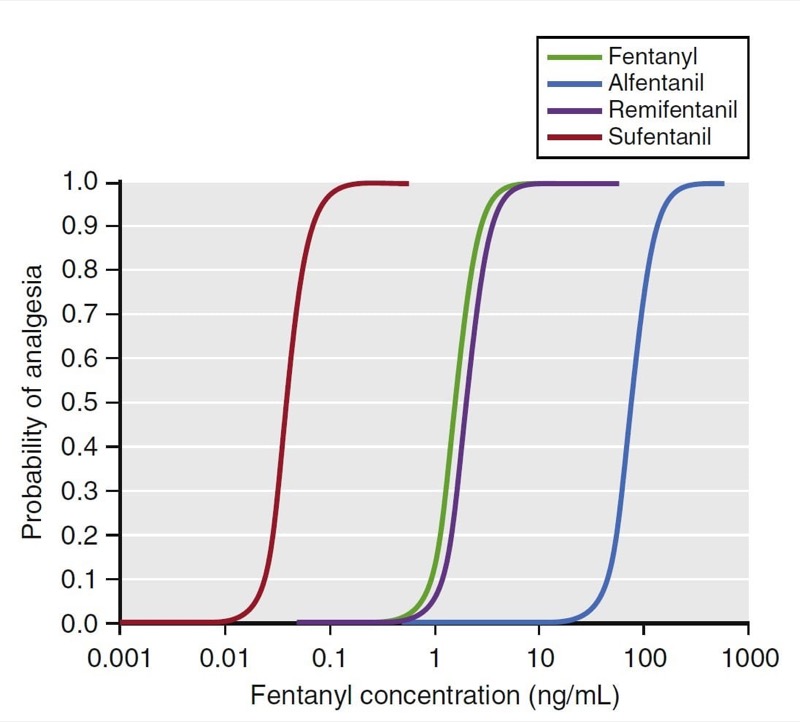
Two important concepts are relevant to this relationship: potency and efficacy. Potency describes the amount of drug required to elicit an effect. The C50 is a common parameter used to describe potency. For drugs that have a concentration-versus-effect relationship that is shifted to the left (small C50), the drug is considered to be more potent, and the reverse is true for drugs that have a concentration-versus-effect relationship shifted to the right. For example, as illustrated in Fig. 21, the analgesia C50 for some of the fentanyl congeners ranges from small for sufentanil (0.04 ng/mL) to large for alfentanil (75 ng/mL). Thus, sufentanil is more potent than alfentanil.

- Fig. 21 Pharmacodynamic models for fentanyl congeners. The C50 for each drug is different, but the slope and maximal effect are similar. (12) (From Miller RD, Cohen NH, Eriksson LI, et al, eds. Miller’s Anesthesia. 8th ed. Philadelphia: Saunders Elsevier; 2015: Fig. 22.)
Efficacy is a measure of drug effectiveness once it occupies a receptor. Similar drugs that work through the same receptor may have varying degrees of effectiveness despite having the same receptor occupancy. For example, with G protein–coupled receptors, some drugs may bind the receptor in such a way as to produce a more pronounced activation of second messengers, causing more of an effect than others. Drugs that achieve maximal effect are known as full agonists and those that have a less than maximal effect are known as partial agonists.
Anesthetic Drug Interactions
An average clinical anesthetic rarely consists of one drug but rather a combination of drugs to achieve desired levels of hypnosis, analgesia, and muscle relaxation. Hypnotics, analgesics, and muscle relaxants all interact with one another such that each drug, when administered in the presence of other drugs, rarely behaves as if it were administered alone. For example, when an analgesic is administered in the presence of a hypnotic, analgesia is more profound with the hypnotic than by itself, and hypnosis is more profound with the analgesic than by itself. Thus, anesthesia is the practice of applied drug interactions. This phenomenon is likely a function of each class of drug exerting an effect on different receptors.
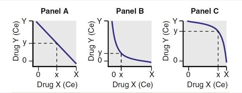
Substantial studies have been performed exploring how anesthetic drugs interact with one another. As illustrated in Fig. 22, interactions have been characterized as antagonistic, additive, and synergistic. When drugs that have an additive interaction are coadministered, their overall effect is the sum of the two individual effects. With antagonistic interactions, the overall effect is less than if the drug combination was additive; with synergistic interactions, the overall effect is greater than if the drug combination was additive.

- Fig. 22 Drug interactions. For two drugs, X and Y, Panel A represents additive, Panel B represents synergistic, and Panel C represents antagonistic interactions. Ce, Effect-site concentration. (From Miller RD, Cohen NH, Eriksson LI, et al, eds. Miller’s Anesthesia. 8th ed. Philadelphia: Saunders Elsevier; 2015:)
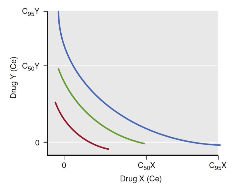
A term used to characterize the continuum of drug concentrations across various combinations of drug pairs (X in combination with Y) is the isobole. The isobole is an isoeffect line for a selected probability of effect. A common isobole is the 50% isobole line. It represents all possible combinations of two-drug effect-site concentrations that would lead to a 50% probability of a given effect. Other isoboles are of more clinical interest. For example, the 95% isobole for loss of responsiveness represents the concentration pairs necessary to ensure a 95% probability of unresponsiveness. Similarly, the 5% isobole represents the concentration pairs having a low likelihood of that effect (i.e., most patients would be responsive). When formulating an anesthetic dosing regimen, dosing an anesthetic to achieve a probability of effect just above but not far beyond the 95% isobole is ideal (Fig. 23).

- Fig. 23 Schematic illustration of isoeffect (isobole) lines. The red, green, and blue lines represent the 50% and 95% isoboles for a synergistic interaction between drugs X and Y. Isoboles represent concentration pairs with an equivalent effect. A set of 5%, 50%, and 95% isoboles can be used to describe the dynamic range of the concentrations for drugs X and Y for a given effect. As with single concentration effect curves, the ideal dosing leads to concentration pairs that are near the 95% isobole. Ce, Effectsite concentration. (From Miller RD, Cohen NH, Eriksson LI, et al, eds. Miller’s Anesthesia. 8th ed. Philadelphia: Saunders Elsevier; 2015)
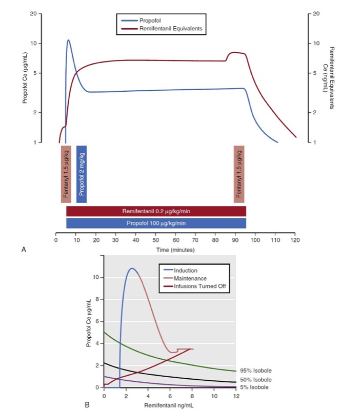
Several researchers have developed mathematical models that characterize anesthetic drug interactions in three dimensions. These models are known as response surface models and include effect-site concentrations for each drug as well as a probability estimate of the overall effect. Fig. 24 presents the propofol remifentanil interaction for loss of responsiveness as published by Bouillon and associates. (13) The response surface presents the full range of remifentanil-propofol isoboles (0% to 100%) for loss of responsiveness. There are two common representations of the response surface model: the three-dimensional plot and the topographic plot. The topographic plot represents a top-down view of the response surface with drug concentrations on the vertical and horizontal axes. Drug effect is represented with selected isobole lines (i.e., 5%, 50%, and 95%).

- Fig. 24 Simulation of a 90-minute total intravenous anesthetic consisting of propofol bolus (2 mg/kg) and infusion (100 μg/kg/min), remifentanil infusion (0.2 μg/kg/min), and intermittent fentanyl boluses (1.5 μg/kg). (A) Resultant effect-site concentrations (Ce) are presented. (B) Predictions of loss of responsiveness are presented on a topographic (top-down) view.
Response surface models have been developed for a variety of anesthetic effects to include responses to verbal and tactile stimuli, painful stimuli, hemodynamic or respiratory effects, and changes in electrical brain activity. For example, with airway instrumentation, response surface models have been developed for loss of response to placing a laryngeal mask airway, (14) laryngoscopy, (15,16) tracheal intubation, (17) and esophageal instrumentation18 for selected combinations of anesthetic drugs. Although many response surface models exist, there are several gaps in available models covering all common combinations of anesthetic drugs and various forms of stimuli encountered in the perioperative environment.
3. SPECIAL POPULATIONS
When formulating an anesthetic, many aspects of patient demographics and medical history need to be considered to determine the correct dose. Such factors include age; body habitus; gender; chronic exposure to opioids, benzodiazepines, or alcohol; presence of heart, lung, kidney, or liver disease; and the extent of blood loss or dehydration. Each of them can dramatically impact anesthetic drug kinetics and dynamics. How some patient characteristics (e.g., obesity) influence anesthetic drug behavior has been studied, whereas other patient characteristics remain difficult to assess (e.g., chronic opioid exposure). The findings are briefly summarized to characterize the pharmacokinetics and pharmacodynamics in a few unique special populations.
Influence of Obesity on Anesthetic Drugs
Obesity is a worldwide epidemic, and overweight patients frequently undergo anesthesia and surgery. Therefore, anesthesia providers should be familiar with the pharmacologic alterations of anesthetics in obese individuals. In general, manufacturer dosing recommendations are scaled to kilograms of actual total body weight (TBW). However, anesthesia providers rarely use mg/kg dosing in obese patients for fear of administering an excessive dose (e.g., a 136-kg patient does not require twice as much drug as a patient of the same height who weighs 68 kg). Accordingly researchers have developed several weight scalars in an attempt to avoid excessive dosing or underdosing in this patient population. Some of these scalars include lean body mass (LBM), ideal body weight (IBW), and fat-free mass (FFM). These scaled weights are usually smaller than TBW in obese patients and thus help prevent excessive drug administration (Fig. 25). Scaled weights have been used in place of TBW for both bolus (mg/kg) and infusion (mg/kg/hr) dosing and also for target-controlled infusions (TCIs).
This section will discuss the pharmacologic alterations of select intravenous anesthetic drugs (propofol, remifentanil, and fentanyl) in obese patients, including shortcomings of weight scalars when used in bolus and continuous infusion dosing.
Propofol
The influence of obesity on propofol pharmacokinetics is not entirely clear. Generally, in obese patients, the blood distributes more to nonadipose than to adipose tissues, resulting in higher plasma drug concentrations in obese patients with mg/kg dosing than in normal patients with less adipose mass. Furthermore, propofol clearance increases because of the increased liver volume and liver blood flow associated with obesity (and increased cardiac output). Changes to volumes of distribution likely influence concentration peaks with bolus dosing, whereas changes in clearance likely influence concentrations during and following infusions. Various weight scalars in propofol bolus and continuous infusion dosing have been studied.
Dosing Scalars for Propofol
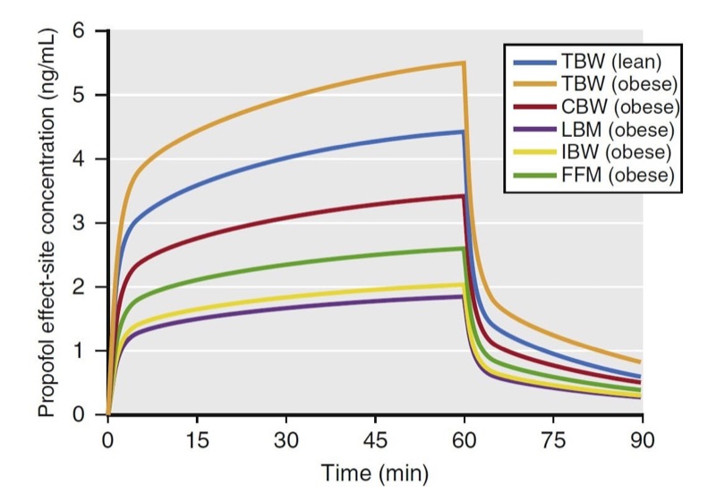
Simulations of an infusion using various weight scalars are presented in Fig. 26. The simulations predict propofol effect-site concentrations from a 60-minute infusion (167 μg/kg/min) in a 176-cm (6-foot)-tall obese (185 kg) and lean (68 kg) male patient. If dosed according to TBW, peak plasma concentrations in the lean and obese individuals are different. The other weight scalars lead to much smaller concentrations with the infusion.
Of the many available dosing scalars, authors recommend LBM24 for bolus dosing (i.e., during induction) and TBW or corrected body weight (CBW) for infusions. (17,25) For continuous infusions, other weight scalars are likely to result in inadequate dosing (most worrisome for LBM).
One concern with using TBW to dose continuous infusions (i.e., μg/kg/min) is drug accumulation. Prior investigations, however, do not support this assumption. Servin and colleagues (22) performed pharmacokinetic analyses of propofol administration to normal and obese patients using TBW and CBW. The CBW was defined as the IBW + 0.4 × (TBW − IBW). (24) They found similar concentrations at eye opening in both groups and absence of propofol accumulation in obese patients. However, some reports suggest that dosing infusions according to CBW may underdose morbidly obese patients. (25)

- Fig. 26 Simulations of propofol plasma concentrations that result from a 60-minute infusion (10 mg/kg/h [167 μg/kg/min]) to a 40-year-old man who is 176 cm tall. Simulations include the following dosing weights: total body weights (TBW) of 68 kg and 185 kg (body mass indices of 22 and 60, respectively) and scaled weights for the 185-kg weight to include Servin’s corrected body weight (CBW), lean body mass (LBM), ideal body weight (IBW), and fat-free mass (FFM). Key points: At the 185-kg weight, when dosed to TBW, the infusion leads to high propofol concentrations, whereas when dosed to IBW or LBM, the infusion leads to low propofol concentrations. When the 185-kg individual is dosed using CBW, it best approximates the propofol concentrations that result from TBW in a lean individual. (From Miller RD, Cohen NH, Eriksson LI, et al, eds. Miller’s Anesthesia. 8th ed. Philadelphia: Saunders Elsevier; 2014)
Other Sedatives
Only limited information is available on the behavior of other sedatives (i.e., midazolam, ketamine, etomidate, and barbiturates) in obese patients. Although not clinically validated in obese patients, bolus doses probably should be based on TBW, and use of other dosing scalars will lead to inadequate effect. In contrast, continuous infusion rates should be dosed to IBW. (26)
Dosing Scalars
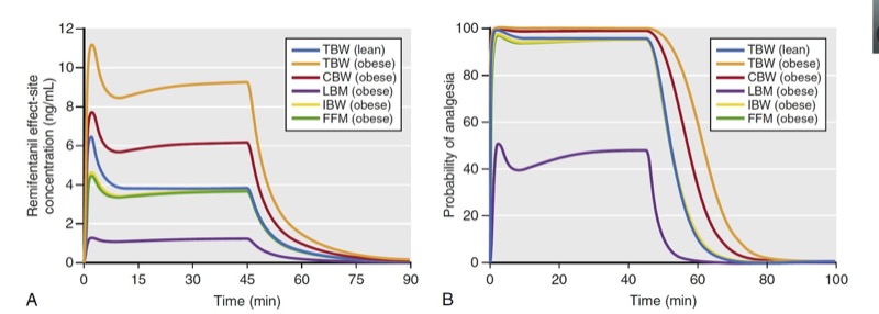
As described with propofol, simulation is used to predict remifentanil effect-site concentrations and analgesic effect for a variety of scaled weights in a 174-cm-tall obese (185 kg, BMI of 60) individual and lean (68 kg, BMI of 22) individual (Fig. 27). Several key points are illustrated in these simulations:
1. For an obese patient, dosing scaled to FFM or IBW resulted in almost identical remifentanil effect-site concentrations as in the lean patient dosed according to TBW. Unlike propofol, dosing remifentanil to CBW (red line, Fig. 27A) leads to higher plasma concentrations compared to levels achieved when dosing to TBW in a lean individual.
2. Dosing scaled to LBM in the obese individual resulted in lower effect-site concentrations than those in a lean individual dosed according to TBW.
3. Dosing the obese individual to TBW was excessive.
4. All dosing scalars, except LBM, provided effect-site concentrations associated with a high probability of analgesia.
As can be appreciated in Fig. 27, LBM has substantial shortcomings in morbidly obese patients. (29) First, dosing remifentanil to LBM leads to plasma concentrations with a low probability of effect compared to the other dosing scalars. Second, with excessive weight (BMI over 40), LBM actually becomes smaller with increasing TBW, making it impractical to use (see Fig. 25). A modified LBM, (24) FFM eliminates the extremely low dosing weight problem. (30) In this simulation, IBW also provides suitable effect-site concentrations, but this may not always be the case when using a weight scalar that is based only on patient height.

- Fig. 27 Simulations of remifentanil effect-site concentrations (A) and analgesic effect (B) that result from a 1-μg/kg bolus and a 60-minute infusion at a rate of 0.15 μg/kg/min to a 40-year-old man who is 176-cm tall. Simulations include the following dosing weights: total body weights (TBW) of 68 kg and 185 kg (body mass indices of 22 and 60, respectively) and scaled weights for the 185-kg weight to include Servin’s corrected body weight (CBW), lean body mass (LBM), ideal body weight (IBW), and fat-free mass (FFM). Remifentanil effect-site concentrations and estimates of analgesic effect were estimated using published pharmacokinetic models. (6,28) Analgesia was defined as loss of response to 30 psi of pressure on the anterior tibia. (From Miller RD, Cohen NH, Eriksson LI, et al, eds. Miller’s Anesthesia. 8th ed. Philadelphia: Saunders Elsevier; 2015)
Fentanyl
Despite widespread use in the clinical arena, relatively little work has explored how obesity affects fentanyl pharmacokinetics. Published fentanyl pharmacokinetic models (31,32) tend to overestimate fentanyl concentrations as TBW increases. (22) Investigators have (20,21) explored ways to improve predictions using published models by modifying demographic data (e.g., either height or weight). Recommendations include use of a modified weight, called the pharmacokinetic mass to improve the predictive performance of one of the many available fentanyl kinetic models.
Other Opioids
Even less information regarding the impact of obesity on drug behavior is available for opioids other than remifentanil and fentanyl. Researchers have studied sufentanil in obese patients and found that its volume of distribution increases linearly with TBW33 and clearance was similar between lean and obese individuals. They recommend bolus dosing using TBW and “prudently reduced” dosing for continuous infusions.
Inhaled Anesthetics
A widely held perception of volatile anesthetics is that they accumulate more in obese than in lean patients and that this leads to prolonged emergence. This concept, however, has not been confirmed. (34) Two phenomena contribute to this observation: first, blood flow to adipose tissue decreases with increasing obesity, (35) and second, the time required to fill adipose tissue with volatile anesthetics is long.
Influence of Increasing Age on Anesthetic Drug Pharmacology
Age is one of the most valuable covariates to consider when developing an anesthetic plan. As with obesity, both remifentanil and propofol can serve as prototypes to understand how age influences anesthetic drug behavior. The influence of age on remifentanil and propofol are characterized in quantitative terms. (1,6,7,36)
With remifentanil, elderly patients require less drug to produce an opioid effect. The effectiveness of reduced doses in older patients is primarily a function of changes in pharmacodynamics but may involve pharmacokinetic changes as well.6 Based on previously published pharmacokinetic and pharmacodynamic models built from measurements over a wide age range, 1,6,7,36 simulations can be performed to explore how age may influence dosing. For example, to achieve equipotent doses in 20- and 80-yearolds, the dose for the 80-year-old should be reduced by 55%. A similar analysis for propofol recommends that the dose for an 80-year-old should be reduced by 65% compared to that of a 20-year-old.
The mechanisms for these changes are not clear, especially for pharmacodynamic changes. One possible source of change in pharmacokinetic behavior may be due to decreased cardiac output. Decreased cardiac output in the elderly (27) results in slower circulation and drug mixing. This may lead to high peak concentrations (27,37) and decreased drug delivery to metabolic organs and reduced clearance. Many intravenous anesthetics (propofol, thiopental, and etomidate) have slower clearance and a smaller volume of distribution. (1) ,(38-40) in the elderly. Beyond age-related changes in cardiac output, other comorbid conditions may reduce cardiovascular function as well. (41) Taking this into account, anesthesia providers often consider a patient’s “physiologic” age instead of solely relying on chronologic age. (42,43) For some older patients, such as those with no significant coexisting disease, normal body habitus, and good exercise tolerance, a substantial reduction in dose may not be warranted.
4. SUMMARY
This chapter reviewed basic principles of clinical pharmacology used to describe anesthetic drug behavior: pharmacokinetics, pharmacodynamics, and anesthetic drug interactions. These principles provide anesthesia practitioners with the information needed to make rational decisions about the selection and administration of anesthetics. From a practical aspect, these principles characterize the magnitude and time course of drug effect, but because of complex mathematics, they have limited clinical utility in everyday practice. Advances in computer simulation, however, have brought this capability to the point of real-time patient care. Perhaps one of the most important advances in our understanding of clinical pharmacology is the development of interaction models that describe how different classes of anesthetic drugs influence one another. This knowledge is especially relevant to anesthesia providers, given that they rarely use just one drug when providing an anesthetic.
5. QUESTIONS OF THE DAY
- In a multicompartment pharmacokinetic model (e.g., for fentanyl bolus administration), what are the three phases that can be distinguished?
- How can a decrement time be used to compare drugs within a drug class? What is the definition of contextsensitive half-time? How does terminal elimination half-life differ from context-sensitive half-time?
- What is the definition of biophase? What is the utility of an effect site compartment in describing anesthetic drug pharmacology?
- What is the difference between antagonistic, additive, and synergistic anesthetic drug interactions? What is an isobole, and how can it be used to determine an appropriate anesthetic regimen?
- How does obesity influence propofol pharmacokinetics? What weight scalar should be used for propofol bolus dose versus propofol infusion dose?
- How does age influence the pharmacology of remifentanil? What are the mechanisms of these age-related changes?